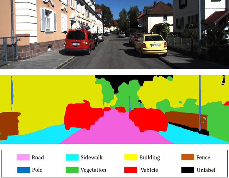
The semantic segmentation task.

The typical goal of semantic segmentation is to assign each pixel in an image to one of a few semantic classes. In the example shown here, each region of the image of a street is labeled as a road, sidewalk, cat, building etc. Oftentimes this problem is reduced to finding a binary pixel mask for each of the possible classes (is this pixel part of a car, or not?), then combining these class-wise masks into a single semantic map.

Applications of semantic segmentation.

Semantic Segmentation has a wide array of applications in many industries, and is an important intermediate step in creating truly intelligent computer-vision systems. In the context of self-driving vehicles, knowing where roads, pedestrians, and other objects are in a single image is a necessary step to determine where these objects are in 3D space. Semantic segmentation is also used in medical image analysis in order to determine the locations of tumors and other defects.

Unfortunately, generalized semantic segmentation is among the hardest computer vision tasks because to predict the class of any single pixel requires high level of contextual knowledge about that pixel and its surroundings. There is almost no way to predict the semantic class of a single pixel using only its RGB values directly. A Blue-Greyish pixel could be part of a sky, a road, a building, a car, a road, or a jacket. It's the challenge of semantic segmentation combined with the clear utility that has us interested in the task.

Motivation

A major challenge of semantic segmentation, or any other machine learning techniques in computer vision is the curse of dimensionality. For a modestly-sized 480x360 color image, there are 480 * 360 * 3 = 518,400 values to consider (one for each RGB value of each pixel). And for semantic segmentation, the output is of size 480 * 360 = 172,800 per class. To train neural networks with data of this dimensionality requires a vast amount of training data and computational power, which are both expensive.

            In short, the goal of our approach is to create a learning-based approach to semantic segmentation that creates a "smaller" predictive model than current convolutional methods. This in turn reduces the amount of training data required to train the model, and speeds up the learning process. This is done by dramatically reducing the dimensionality of the input to our predictive model.

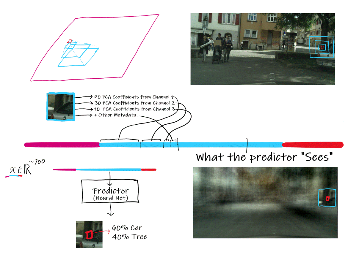
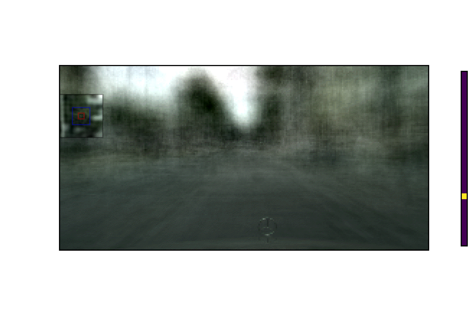
Multiscale Sliding Windows

            One way that we accomplish this is by creating a model that makes a prediction only about a small "chunk" of an image. In our case, we predict the semantic composition of only a 32x32 chunk of a high-resolution image. However, in order to make a prediction about that small chunk, it helps to also know the visual "context" of the area surrounding that chunk. This context is captured by using a multiscale "pyramid" of progressively larger but lower-fidelity chunks surrounding the "core" chunk we wish to make a prediction on.

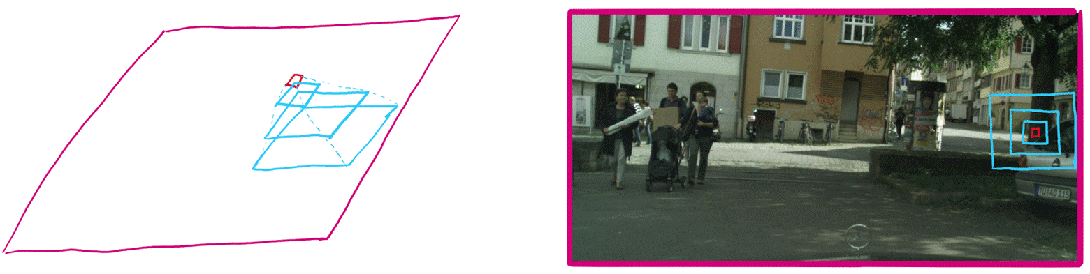
            In order to perform semantic segmentation on the whole image, we then slide this pyramid across the whole image, giving us a semantic prediction of every 32x32 subblock.

Texture Dimensionality Reduction with PCA

As mentioned, image data is inherently very high-dimensional. Limiting the prediction inputs to the images of the multiscale pyramid helps reduce this dimensionality somewhat, but not enough to make a truly small model. So, we use Principle Component Analysis to reduce the input dimensionality even further.

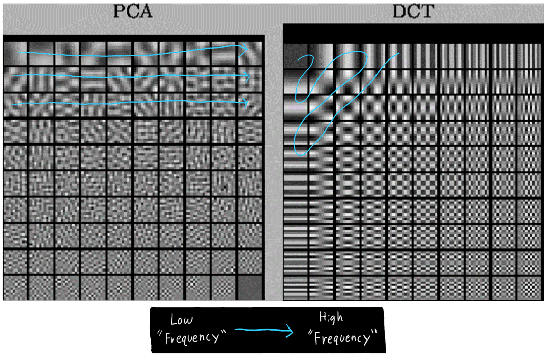
Consider a single 32x32 black & while image. Similar to how we can use the fourier transform / discrete cosine transform to perform a "basis" transformation, giving us the original 32x32 image in different basis coefficients, we can also use PCA to get different basis coefficients for the image. We can then "drop" most of these basis coefficients, obtaining a compact "representation" of the original 32x32 image. If we want to perform a prediction about this 32x32 image, we can use maybe 90 of the most important PCA coefficients instead of the whole 1024 pixel values.

Color Dimensionality Reduction with PCA

            Beyond using PCA to reduce the dimensionality of the "Texture" information of an image sub-block, we can also use PCA to reduce the dimensionality of the color information of each image. Images are typically thought of as having red, green, and blue channels. To dimensionality-reduce an image, we could apply the PCA texture encoding to the red, green, & blue channels of an image. However, if you apply PCA to the RGB values of an image, you get a more efficient way to represent an image. 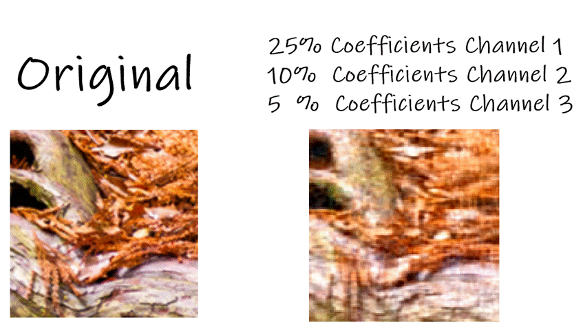You get three new channels, specific to that image, where the first channel is "most important", the second one less important than the first channel, and the last channel least important. For example, this small image of some tree roots with mulch is well approximated when using only ⅔ "PCA" channels.

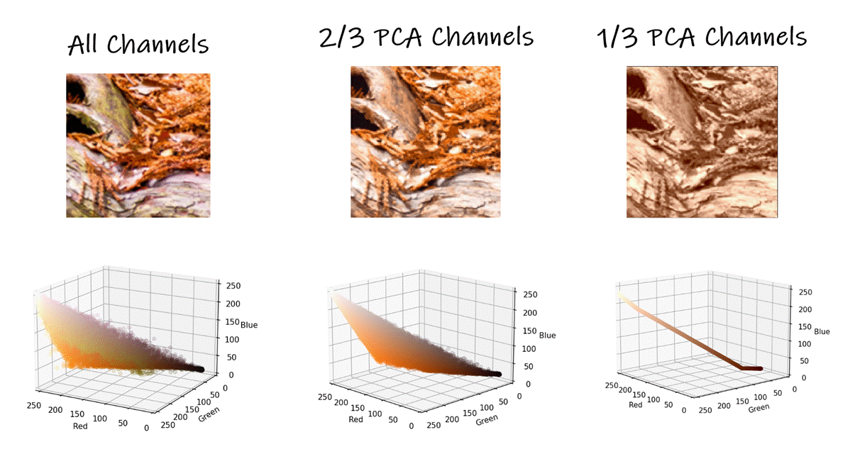
            Instead of applying PCA texture dimensionality reduction to the red, green, and blue channels, we apply it to the 3 custom "PCA" channels. Because we know that the channels are ordered by importance, we encode the most texture information about the first channel, and less in the other two channels.

Putting it together: the encoding.

In order to predict the semantic composition of a single "core" block, we encode the visual information of that block, and larger blocks in that multiscale pyrymic into a single vector, reducing the dimensionality of the input by a large margin.

Cityscapes Dataset

Utilize the cityscapes dataset to classify objects within the city, such as cars, foliage, sky, road, and signs. Our inspiration for using this being self-driving cars.

Constraints

No corners for now. Also we just predict the semantic composition of a core block, not which pixels actually belong to which class.

Model Size

Our model size contains a total of 47,998 parameters, which is tiny in comparison to UNET's massive 2,060,424 parameters in their model.

Training Time

Given this massive difference in the number of parameters, the training times are also vastly different. Our neural network could be trained within 20 minutes while utilizing 30% of a laptop processor, meanwhile UNET's pixel-wise segmentation model used a graphics card while still taking 400 minutes to train.

Inference/ Prediction Time

At this moment, it takes 60 seconds in order to process and predict the labels on the image.

Accuracy

The accuracy of our 47,998 parameter model has an accuracy of 82.79%. Our 203,630 parameter model has an accuracy of 90.08%, and our 845,982 has an accuracy of 93.04%. Each model was only trained for 20 minutes.

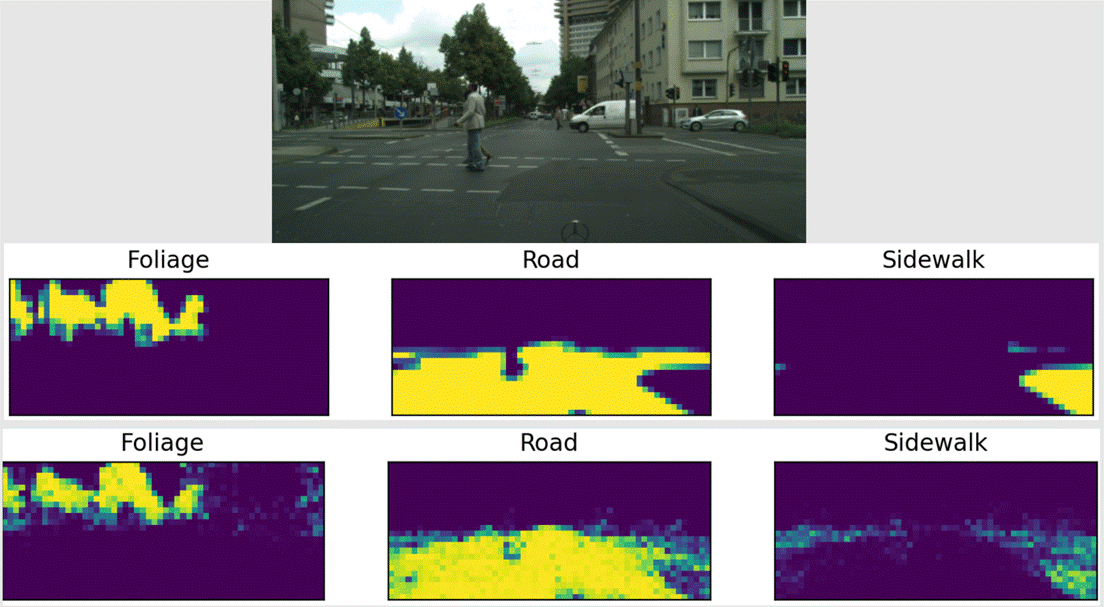
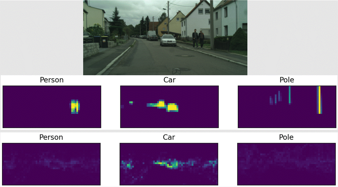
The pictures below are examples of the model in action using the 47,998 parameter model, with the top three being the actual labels taken from the image, and the bottom three being the ones our model had predicted.

Successes:

Areas of improvement:

Inference Time is slow

Inference time is slow with it taking 60 seconds to predict all of the labels within the large image.

Corners

We want our method of image segmentation to also work on corners, at this moment it cannot reach the corners due to the lack of information received from our current algorithm. 

Follow Up with a coarse -> fine step.

We would like to refine our coarse segmentation to a pixel-wise, fine segmentation as to have more data to work with. Having the coarse segmentation limits our ability to have a completely accurate prediction due to losing some fine information which is important at times.